
TL;DR
-
A data warehouse is a columnar, query-optimized store for historical analytics - not for transactional application writes. It answers "revenue by region by quarter" in seconds, not hours.
-
OLAP (Online Analytical Processing) enables fast aggregations across millions of rows - slice by region, time, and product in sub-second queries, because columnar engines read only the columns a query touches.
-
Star schema is the default modeling pattern - fact tables (metrics at a defined grain) surrounded by denormalized dimension tables (context). Grain is the single most important modeling decision.
-
Warehouses are fed by ETL/ELT pipelines from operational systems, SaaS tools, and data lakes - the modern default is ELT with dbt transforming raw staging data inside the warehouse.
-
Governed metrics in the warehouse are the source of truth for dashboards - one tested definition of "revenue" in a dbt model, not twelve conflicting spreadsheet formulas.
Quick Decision Guide
| Your situation | Use |
|---|---|
| BI dashboards, governed SQL metrics, finance reporting | Data warehouse (Snowflake, BigQuery, Redshift, Databricks SQL) |
| Raw, unstructured, or ML training data at scale | Data lake (S3/GCS + Parquet) |
| One platform for both BI and ML on open table formats | Lakehouse (Delta Lake, Iceberg) |
| Single-node analytics, local development, embedded OLAP | DuckDB |
| Federated SQL over lake + warehouse + operational stores | Trino |
Who this guide is for
- Data engineers building the pipelines that load and model warehouse tables.
- Analytics engineers writing dbt models, tests, and metric definitions.
- Backend/ML engineers who consume warehouse tables for features and reporting and need to understand grain, SCD, and cost behavior.
- Architects and tech leads choosing between warehouse, lake, and lakehouse platforms.
Learning Path
Prerequisites: ETL - warehouses are the destination most pipelines serve.
Next topics: Data Lakes · Lakehouse
Estimated time: 55 min · Difficulty: Intermediate
On this page
- Why This Matters
- The Problem Warehouses Solve
- How We Got Here
- What Is a Data Warehouse?
- How Data Warehouses Work
- Architecture
- Step-by-Step Flow
- Real Production Example
- Design Decisions
- Comparisons
- Common Mistakes
- Where It Breaks Down
- When NOT to Use a Data Warehouse
- Running in Production
- Production Checklist
- Related Guides
- Interview Questions
- Key Takeaways
- FAQs
- References
Why This Matters
Your CEO asks: "What was Q2 revenue by region, broken down by product line, compared to last year?" Answering this from production PostgreSQL means expensive JOINs across tables designed for order inserts, not billion-row aggregations - and running it during business hours risks slowing checkout for real customers. Running it on raw S3 files requires writing Spark jobs and hoping the schema hasn't drifted.
A data warehouse answers this in seconds with a SQL query against pre-modeled tables. Finance, product, marketing, and operations teams depend on warehouse-backed dashboards - Snowflake, BigQuery, Redshift, Databricks SQL - for daily decisions.
If you build data pipelines, the warehouse is usually the destination your ETL serves. If you build analytics or AI features, the warehouse provides curated, governed inputs. Understanding warehouse architecture prevents the "three different revenue numbers" problem that destroys organizational trust in data.
Engineering Insight
A data warehouse is not just a big database - it is a contract. When "revenue" is one tested, documented dbt model, every dashboard agrees. When it is twelve ad-hoc queries, every executive meeting starts with an argument about whose number is right.
The Problem Warehouses Solve
Operational databases (OLTP) optimize for row-level reads and writes: insert an order, look up a user, update inventory. Analytics needs the opposite:
| OLTP (Application DB) | OLAP (Data Warehouse) |
|---|---|
| Many small transactions per second | Few large read queries |
| Normalized schema (3NF) to avoid update anomalies | Denormalized star/snowflake schema for simple joins |
| Current state only | Historical snapshots and change tracking |
| Row-oriented storage (read whole rows) | Column-oriented storage (read only needed columns) |
| Single-record lookups by primary key | Aggregations over millions or billions of rows |
| Millisecond latency, high concurrency | Second-to-minute latency, moderate concurrency |
Without a warehouse, organizations fall into three failure modes:
-
Everyone queries production. Analysts run 40-second GROUP BY queries against the same PostgreSQL that serves customers. One bad query locks tables and pages the on-call engineer.
-
Everyone exports CSVs. Data is stale the moment it lands in a spreadsheet, and every export applies slightly different filters, so no two reports match.
-
Everyone builds shadow metrics. Marketing defines "active user" one way, product another, finance a third. Nobody can reconcile the numbers, and trust in data collapses.
Warehouses provide one governed place where data from CRM, billing, product databases, and SaaS tools is integrated, historized, and modeled - so "revenue" means the same thing everywhere it appears.
How We Got Here
The warehouse concept is over three decades old, but the economics changed completely when cloud platforms separated storage from compute.
Diagram: Evolution of the data warehouse
timeline
    title From on-prem appliances to cloud elasticity
    1992-2000 : Kimball vs Inmon
              : Star schema and dimensional modeling
              : Enterprise DW on Oracle and Teradata
    2000-2010 : MPP appliances
              : Netezza and Teradata scale-out
              : Columnar storage (Vertica)
    2012-2016 : Cloud warehouses
              : Redshift launches (2012)
              : Snowflake separates storage and compute
              : BigQuery serverless model
    2016-2021 : ELT era
              : dbt makes SQL transformation standard
              : Fivetran and Airbyte commoditize ingestion
    2021-2026 : Convergence
              : Lakehouse (Delta and Iceberg) blurs boundaries
              : Warehouses read open table formats
              : DuckDB brings OLAP to a laptop
Each era removed a constraint: modeling discipline (Kimball), scale (MPP), elasticity (cloud), transformation tooling (dbt), and format lock-in (open tables).
Kimball vs Inmon (1990s). Ralph Kimball advocated bottom-up dimensional modeling - build star-schema data marts per business process, conform dimensions across them. Bill Inmon advocated top-down - build a normalized enterprise warehouse first, derive marts from it. Kimball's approach won most adoption because it delivers value per business process instead of after a multi-year enterprise model.
MPP appliances (2000s). Teradata and Netezza sold massively parallel processing hardware: queries fan out across nodes, each scanning its shard. Powerful but capital-intensive - capacity planning meant buying racks years ahead.
Cloud separation of storage and compute (2010s). Redshift (2012) moved MPP to rented instances. Snowflake and BigQuery went further: data lives in cheap object storage while stateless compute clusters spin up on demand and scale independently. You stopped paying for idle capacity, and multiple teams could query the same data with isolated compute.
ELT and dbt (late 2010s). With cheap warehouse compute, transformation moved inside the warehouse: load raw data first, transform with SQL. dbt added software-engineering discipline - version control, tests, documentation, lineage - and became the de facto transformation standard.
Convergence (2020s). Lakehouse formats (Delta Lake, Apache Iceberg) brought warehouse features to lakes; warehouses in turn learned to query open formats directly. DuckDB made columnar OLAP an embeddable library, and Trino made it a federated query layer.
What Is a Data Warehouse?
A data warehouse is a centralized repository that stores integrated data from multiple sources, optimized for analytical queries and reporting. Inmon's classic definition names four characteristics, all still accurate:
-
Subject-oriented - Organized by business concepts (customers, orders, revenue), not by application tables.
dim_customerunifies CRM contacts, billing accounts, and product users. -
Integrated - Data from CRM, billing, and product databases is unified with consistent definitions, keys, and units. "Country" is ISO codes everywhere, not
USin one source andUnited Statesin another. -
Time-variant - The warehouse keeps history. Slowly changing dimensions (SCD) track how attributes change: when a customer moves from
SMBtoEnterprisesegment, both states are preserved with validity dates. -
Non-volatile - Data arrives via controlled ETL/ELT loads, appended or merged in batches. The warehouse is not a live application backend that mutates row by row.
Modern cloud warehouses add elastic compute, separation of storage and compute, automatic optimization, and near-zero administration compared to on-premise appliances (Teradata, Netezza). The physical engine changed; the modeling principles did not.
How Data Warehouses Work
Three mechanisms make a warehouse fast and trustworthy: columnar OLAP execution, dimensional (star schema) modeling, and controlled ingestion.
OLAP and columnar execution
OLAP (Online Analytical Processing) describes workloads that aggregate large datasets across multiple dimensions:
-- Classic OLAP query: slice and dice
SELECT
    d_region.region_name,
    d_product.category,
    SUM(f_revenue.amount) AS total_revenue,
    COUNT(DISTINCT f_revenue.customer_key) AS unique_customers
FROM fact_revenue f_revenue
JOIN dim_date d_date ON f_revenue.date_key = d_date.date_key
JOIN dim_region d_region ON f_revenue.region_key = d_region.region_key
JOIN dim_product d_product ON f_revenue.product_key = d_product.product_key
WHERE d_date.fiscal_quarter = '2026-Q2'
GROUP BY 1, 2
ORDER BY total_revenue DESC;
The standard OLAP operations:
| Operation | Meaning | Example |
|---|---|---|
| Slice | Filter one dimension | Q2 only |
| Dice | Filter multiple dimensions | Q2 + EMEA region |
| Roll-up | Aggregate to higher level | Daily → monthly revenue |
| Drill-down | Decompose aggregate | Region → country → city |
| Pivot | Rotate dimensions | Products as columns, months as rows |
Columnar storage makes these fast. A row store must read every full row to sum one column; a column store reads only amount and date_key, compressed together because similar values sit adjacent. Combined with partition pruning (skip files outside the date filter) and vectorized execution, this is why a billion-row aggregation finishes in seconds.
Star schema and dimensional modeling
Star schema is the default warehouse design - a central fact table connected to dimension tables like a star.
Fact tables store measurable events - one row per business event at a defined grain:
| Fact Table | Grain | Metrics |
|---|---|---|
fact_orders |
One row per order line | amount, quantity, discount |
fact_pageviews |
One row per page view | duration_sec, is_bounce |
fact_subscriptions |
One row per subscription per month | mrr, is_churned |
Grain is sacred. Every metric on a fact table must be valid at that grain. If grain is order-line, never store order-level totals on the same row without careful semi-additive handling - summing them double-counts.
Dimension tables provide context for slicing facts - wide, denormalized, human-readable:
| Dimension | Attributes |
|---|---|
dim_date |
fiscal_quarter, is_weekend, holiday_name |
dim_customer |
segment, signup_date, country |
dim_product |
category, brand, sku |
Dimensions use surrogate keys - warehouse-generated integers (customer_key) independent of source-system IDs. Source IDs change when systems merge records or migrate; surrogate keys also enable SCD Type 2, where one customer has multiple rows over time.
Tip
Pre-join dimension attributes analysts filter on. A
dim_productwithcategoryandsubcategorycolumns beats a 4-table normalized snowflake for dashboard performance and analyst sanity.
How data gets in
Warehouses are populated by ETL or ELT pipelines:
- Extract - Pull from sources: operational databases (CDC or snapshots), SaaS APIs (Fivetran, Airbyte), and data lake files.
- Load raw - Land data in a
staging/rawschema with minimal transformation - preserve source truth. - Transform - dbt models build staging views, then dimensions and facts with business logic, entirely in warehouse SQL.
- Test - Uniqueness, not-null, referential integrity, and metric reconciliation tests run before marts are exposed.
- Serve - BI tools query analytics marts only, never raw staging.
The modern pattern is ELT: because cloud warehouse compute is elastic and cheap relative to engineering time, you load first and transform in SQL, version-controlled in Git. Heavy pre-warehouse processing (parsing large semi-structured files, ML feature pipelines) still happens in Spark or on Databricks before load.
Architecture
A production warehouse is organized in layers, each with a clear contract: raw data enters staging untouched, dimensional models apply business logic, and marts serve consumers.
Diagram: Warehouse layered architecture
flowchart LR
    subgraph Sources
        DB[(App databases)]
        SaaS[SaaS APIs]
        Lake[(Data lake)]
    end
    subgraph Warehouse
        STG[staging schema<br/>raw landed data]
        subgraph Core [analytics core]
            DIM[dim_customer<br/>dim_product<br/>dim_date]
            FACT[fact_orders<br/>fact_subscriptions]
        end
        MART[marts<br/>finance / product / marketing]
    end
    BI[BI dashboards<br/>Looker · Tableau]
    DB -->|CDC / Fivetran| STG
    SaaS -->|Airbyte| STG
    Lake -->|curated loads| STG
    STG -->|dbt models + tests| DIM
    STG -->|dbt models + tests| FACT
    DIM --> MART
    FACT --> MART
    MART --> BI
Raw data flows one direction: staging → dimensions and facts → marts. Dashboards query marts only; staging is never exposed.
Staging layer. One table per source object, loaded as-is (or lightly typed). Staging is disposable and re-loadable - if a transformation bug ships, you rebuild downstream models from staging without re-extracting.
Core dimensional layer. dbt models join, deduplicate, and apply business logic to produce conformed dimensions and fact tables. This is where surrogate keys are generated, SCD Type 2 history is maintained, and grain is enforced.
Marts layer. Department-facing schemas (finance, product, marketing) exposing curated, documented tables and pre-aggregations. Access control lives here: finance sees revenue detail, marketing sees anonymized aggregates.
The star schema at the heart of the core layer looks like this - the diagram below shows fact_orders at the center with four dimensions radiating outward, which is exactly the "star" shape the pattern is named for:
Diagram: Star schema for order analytics
erDiagram
    DIM_DATE ||--o{ FACT_ORDERS : "date_key"
    DIM_CUSTOMER ||--o{ FACT_ORDERS : "customer_key"
    DIM_PRODUCT ||--o{ FACT_ORDERS : "product_key"
    DIM_REGION ||--o{ FACT_ORDERS : "region_key"
    FACT_ORDERS {
        bigint order_line_id PK
        int date_key FK
        int customer_key FK
        int product_key FK
        int region_key FK
        decimal amount
        int quantity
        decimal discount
    }
    DIM_DATE {
        int date_key PK
        date full_date
        string fiscal_quarter
        boolean is_weekend
    }
    DIM_CUSTOMER {
        int customer_key PK
        string customer_id
        string segment
        string country
        date valid_from
        date valid_to
        boolean is_current
    }
    DIM_PRODUCT {
        int product_key PK
        string sku
        string category
        string brand
    }
    DIM_REGION {
        int region_key PK
        string region_name
    }
One fact table at atomic grain (order line), four denormalized dimensions. Note valid_from/valid_to/is_current on dim_customer - that is SCD Type 2 history.
Every OLAP query in this guide follows the same shape you see in this star: filter on dimension attributes, join to the fact on surrogate keys, aggregate the fact's numeric columns. Because the fact table stores only compact integer keys and metrics, it stays narrow and scans fast even at billions of rows, while the wide descriptive columns live once in each small dimension.
Step-by-Step Flow
Here is what a nightly ELT run looks like end to end with an orchestrator, an ingestion tool, and dbt:
Diagram: Nightly ELT pipeline with dbt
sequenceDiagram
    participant Orch as Orchestrator (Airflow/Dagster)
    participant Ing as Ingestion (Fivetran/Airbyte)
    participant WH as Warehouse (staging)
    participant dbt as dbt
    participant Marts as Marts
    participant BI as BI tool

    Orch->>Ing: 1. Trigger sync (02:00 UTC)
    Ing->>WH: 2. Load incremental rows to staging
    Ing-->>Orch: 3. Sync complete + row counts
    Orch->>dbt: 4. dbt run (staging → dims → facts)
    dbt->>WH: 5. Build dim_customer (SCD merge)
    dbt->>WH: 6. Incremental MERGE into fact tables
    Orch->>dbt: 7. dbt test
    dbt-->>Orch: 8. Tests pass (unique, not_null, relationships)
    Orch->>Marts: 9. Promote marts (swap / publish)
    BI->>Marts: 10. Dashboards query fresh marts
    Note over Orch,BI: On test failure: halt promotion, alert, dashboards keep yesterday's data
Tests gate promotion: a failed uniqueness test stops bad data from reaching dashboards - stale data beats wrong data.
The corresponding dbt incremental model for the fact table:
-- models/marts/fact_orders.sql
{{ config(
    materialized='incremental',
    unique_key='order_line_id',
    incremental_strategy='merge',
    partition_by={'field': 'order_date', 'data_type': 'date'}
) }}

SELECT
    s.order_line_id,
    d.date_key,
    c.customer_key,
    p.product_key,
    s.amount,
    s.quantity,
    s.discount
FROM {{ ref('stg_order_lines') }} s
JOIN {{ ref('dim_date') }} d ON s.order_date = d.full_date
JOIN {{ ref('dim_customer') }} c
    ON s.customer_id = c.customer_id AND c.is_current
JOIN {{ ref('dim_product') }} p ON s.product_id = p.product_id
{% if is_incremental() %}
WHERE s.updated_at > (SELECT MAX(updated_at) FROM {{ this }})
{% endif %}
And the tests that gate promotion:
# models/marts/schema.yml
models:
  - name: fact_orders
    columns:
      - name: order_line_id
        tests: [unique, not_null]
      - name: customer_key
        tests:
          - not_null
          - relationships:
              to: ref('dim_customer')
              field: customer_key
Key operational details:
- Watermarks, not full reloads. The
is_incremental()filter processes only rows changed since the last run - a billion-row fact table ingests thousands of new rows, not everything. - MERGE for late-arriving updates. Source rows that change after first load (order cancellations, refunds) are upserted by
unique_key, not duplicated. - Idempotency. Re-running a failed job produces the same result - MERGE semantics make retries safe.
Real Production Example
A subscription SaaS company models MRR (monthly recurring revenue) in Snowflake. The two hard problems are (1) customer attributes change over time and finance needs history, and (2) MRR must have exactly one definition.
SCD Type 2 dimension. When a customer's segment changes (SMB → Enterprise), finance must attribute past revenue to the segment the customer was in at the time. Overwriting the segment would silently rewrite history. SCD Type 2 keeps every version with validity windows:
-- dim_customer with SCD Type 2 for segment changes
CREATE TABLE analytics.dim_customer AS
SELECT
    customer_id,
    customer_name,
    segment,
    country,
    valid_from,
    valid_to,
    is_current
FROM staging.customer_snapshots;

-- fact_subscriptions - grain: one row per customer per month
CREATE TABLE analytics.fact_subscriptions AS
SELECT
    d.date_key,
    c.customer_key,
    p.product_key,
    s.mrr_amount,
    s.is_active,
    s.is_churned
FROM staging.subscription_monthly s
JOIN analytics.dim_date d ON s.month_start = d.full_date
JOIN analytics.dim_customer c
    ON s.customer_id = c.customer_id
    AND s.month_start >= c.valid_from
    AND s.month_start < COALESCE(c.valid_to, '9999-12-31')
JOIN analytics.dim_product p ON s.product_id = p.product_id;
The range join against valid_from/valid_to picks the dimension version that was current in each subscription month - so a customer who upgraded to Enterprise in March contributes January and February MRR to SMB, correctly.
One metric definition. The finance dashboard queries fact_subscriptions joined to dim_date and dim_customer. The MRR definition - which subscription states count, how proration works, how churn is flagged - lives in one dbt model with tests, not in twelve spreadsheets. In practice the project is a dbt DAG from sources through staging to marts:
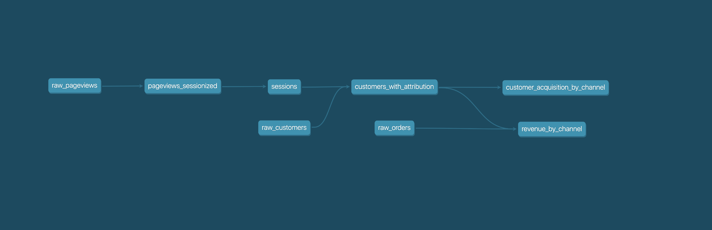
Source: dbt Labs
Results at this company after migrating from spreadsheet reporting: month-end close queries dropped from hours of manual reconciliation to a dashboard refresh, and the "which MRR number is right?" debate disappeared because there is only one MRR model - tested nightly for uniqueness on (customer_key, date_key) and reconciled against the billing system total within 0.1%.
Design Decisions
| Decision | Option A | Option B | When to choose |
|---|---|---|---|
| Modeling | Star schema | Data Vault | Star for most BI; Data Vault for heavy regulatory audit trails across many volatile sources |
| Load pattern | ELT (transform in warehouse) | ETL (transform before load) | ELT with dbt as default; ETL when data must be cleansed/masked before it may land |
| Refresh | Incremental MERGE | Full refresh | Incremental for large facts; full refresh for small dimensions (simpler, self-healing) |
| Materialization | Tables | Views / materialized views | Tables for production dashboards; views for exploratory or cheap-to-compute layers |
| Grain | Atomic (line-item) | Pre-aggregated | Atomic for flexibility; add aggregate tables when query cost or latency demands it |
| SCD handling | Type 1 (overwrite) | Type 2 (history rows) | Type 2 whenever anyone asks "as of" questions; Type 1 for corrections only |
| Compute sizing | Fixed warehouse | Auto-scaling / serverless | Fixed for predictable nightly loads; auto-scale for spiky ad-hoc analyst traffic |
| Platform | Snowflake | BigQuery / Redshift / Databricks SQL | Ecosystem fit, existing cloud, pricing model for your workload (see Comparisons) |
Common patterns
- Conformed dimensions. One
dim_customershared by every fact table, so "customers" filters identically across revenue, support, and product dashboards. - Date spine. A generated
dim_datecovering all dates (including no-activity days) so time series don't silently skip days. - Aggregate/rollup tables. Pre-computed daily or monthly summaries on top of atomic facts for the hottest dashboards - built by dbt, never hand-maintained.
- Semantic layer. Metric definitions (dbt metrics, LookML) on top of marts so BI tools consume governed measures instead of raw SQL.
Comparisons
OLTP vs OLAP
| OLTP database | OLAP warehouse | |
|---|---|---|
| Purpose | Run the application | Analyze the business |
| Query shape | Point reads/writes by key | Scans + aggregations |
| Storage | Row-oriented | Columnar |
| Schema | Normalized (3NF) | Star / dimensional |
| Data | Current state | Full history |
| Examples | PostgreSQL, MySQL | Snowflake, BigQuery, Redshift |
Snowflake vs BigQuery vs Redshift vs Databricks SQL
| Snowflake | BigQuery | Redshift | Databricks SQL | |
|---|---|---|---|---|
| Pricing model | Per-second compute credits | On-demand per TB scanned, or slots | Instance-hours (RA3) / serverless RPU | DBU-based clusters / serverless |
| Storage/compute separation | Yes, independent scaling | Yes, fully serverless | Partial (RA3 managed storage) | Yes (lake-backed) |
| Ops burden | Low | Lowest (no clusters) | Highest (tuning, WLM) | Low-medium |
| Semi-structured data | Strong (VARIANT) |
Strong (JSON, nested/repeated) | Adequate (SUPER) | Strong (open formats) |
| Open table formats | Iceberg support | BigLake / Iceberg support | Via Spectrum / lake | Native Delta, Iceberg via UC |
| Best fit | Multi-cloud, workload isolation | GCP shops, spiky ad-hoc | AWS shops with steady load | Lakehouse-first, ML + BI on one platform |
Cost behavior differs fundamentally: BigQuery on-demand charges per byte scanned (a careless SELECT * on a wide table is expensive), Snowflake charges per second a warehouse runs (idle-but-running clusters are the waste), and Redshift provisioned charges per hour regardless of use. Model your actual workload before choosing on price.
Star vs snowflake schema vs Data Vault
| Star | Snowflake schema | Data Vault | |
|---|---|---|---|
| Dimension shape | Denormalized, wide | Normalized into sub-tables | Hubs, links, satellites |
| Query complexity | Simplest (1 join per dim) | More joins | Highest (query from views) |
| Storage | Some redundancy | Minimal redundancy | Higher (full history everywhere) |
| Change handling | SCD on dimensions | SCD, more granular | Every change appended by design |
| Best for | Most BI workloads | Deep hierarchies, storage-constrained | Audit-heavy, many volatile sources |
Default to star. Storage is cheap; analyst time and query simplicity are not. Data Vault earns its complexity only when auditability across dozens of changing sources is a hard requirement - and it still needs star-schema marts on top for BI.
Warehouse vs data lake vs lakehouse
| Warehouse | Data lake | Lakehouse | |
|---|---|---|---|
| Data | Structured, modeled | Anything, raw | Structured + semi-structured on open formats |
| Schema | On write | On read | On write with evolution |
| Consumers | BI, SQL analysts | Data/ML engineers | Both |
| ACID transactions | Yes | No | Yes (Delta/Iceberg) |
| Cost profile | Compute premium | Cheapest storage | Lake storage + engine compute |
Decision tree: Warehouse, lake, or lakehouse?
flowchart TD
    Q1{Primary workload?} -->|Governed BI + SQL metrics| Q2
    Q1 -->|Raw / unstructured / ML training| Lake[Data lake]
    Q1 -->|Both BI and ML equally| LH[Lakehouse]
    Q2{Data volume + team size?} -->|Small / local / embedded| Duck[DuckDB]
    Q2 -->|Org-wide, multiple teams| WH[Cloud warehouse]
    Lake -->|Need SQL over lake files| Trino[Trino / federated SQL]
    WH -->|Later: ML needs raw data too| LH
Most mature organizations run a lake for raw data and a warehouse (or lakehouse) for governed analytics - the choice is emphasis, not exclusivity.
Common Mistakes
-
Wrong grain on fact tables. Mixing order-level and line-level metrics in one table produces double-counting. Declare grain in the model description and test it (
uniqueon the grain columns). -
Querying staging tables in dashboards. Staging is raw and disposable. The first time an analyst builds a board on
staging.orders_raw, you can never safely rebuild it. Production marts only. -
No surrogate keys. Using source-system IDs directly breaks when sources merge records or migrate. Generate
customer_keyindependent of the CRM ID - and it's required for SCD Type 2 anyway. -
Ignoring slowly changing dimensions. Customer segments change; overwriting (Type 1) silently rewrites the history finance reports on. Decide SCD strategy per dimension before the first load.
-
Fan-out joins. Joining facts to a table at finer grain multiplies metrics: one $100 order becomes $500 after joining five promo-code rows. Test row counts before and after joins.
-
Three definitions of revenue. Metric logic scattered across BI tools drifts apart. Define once in dbt, document, test, and point every tool at the same model.
-
SELECT *on pay-per-scan platforms. On BigQuery on-demand, scanning all columns of a wide table costs real money every dashboard refresh. Select only needed columns; the columnar engine rewards you twice. -
No cost guardrails. One analyst's accidental cross join on Snowflake can burn a month of credits overnight. Set resource monitors, query timeouts, and per-team warehouses from day one.
Where It Breaks Down
Unstructured data. Warehouses excel at structured analytics. Text, images, audio, and raw JSON event blobs belong in data lakes - the warehouse stores extracted features or aggregates, not the raw payloads.
Real-time requirements. Nightly (or hourly) batch loads mean dashboards lag reality. Sub-second operational dashboards - live fraud counters, inventory levels - need streaming systems or pre-computed caches, not a warehouse query per page load.
Cost at scale. Full table scans on petabyte facts are expensive on every platform. Without partition pruning, clustering, and aggregate tables, the monthly bill grows faster than the data.
Schema rigidity for exploration. New data sources wait for modeling before analysts can touch them. Teams that need fast exploration land raw data in the lake first and promote to modeled warehouse tables once questions stabilize.
High-concurrency serving. A warehouse serving thousands of concurrent low-latency application queries (user-facing analytics embedded in your product) hits concurrency limits and cost cliffs - purpose-built serving layers or pre-computed results handle that tier.
When NOT to Use a Data Warehouse
-
As an application backend. OLTP workloads - single-row lookups, high-frequency writes, transactional integrity per request - belong in PostgreSQL/MySQL. Warehouse write paths are batch-oriented.
-
For sub-second operational dashboards. Live ops screens need streaming aggregation or caches; warehouse query latency is seconds.
-
For raw ML training data. Petabytes of images, logs, or text are cheaper and more flexible in a lake; train from object storage with Spark and store only features/labels in the warehouse.
-
When the data fits on a laptop. A startup with gigabytes of data does not need Snowflake. DuckDB over Parquet files delivers full columnar OLAP with zero infrastructure - migrate when concurrency and governance demand it.
-
When you only need federation. If the goal is SQL across existing stores without copying data, Trino queries lakes, warehouses, and operational databases in place.
-
Before anyone asks analytical questions. A warehouse without consumers is pure cost. Build it when dashboard and metric demand exists, not speculatively.
Running in Production
Important
One definition per metric. "Revenue" documented in dbt with tested logic - not redefined in every Looker explore.
| Dimension | Consideration |
|---|---|
| Scaling | Separate compute per workload (loading vs BI vs data science) so a heavy backfill never slows dashboards. Size for the p95 workload, auto-suspend idle compute. |
| Cost | Resource monitors / budgets with alerts; per-team attribution via warehouse/project tagging; review top-10 most expensive queries weekly. Partition + cluster large facts to cut scan volume. |
| Freshness | Publish SLAs per mart (e.g., finance marts by 06:00 UTC). Monitor with dbt source freshness checks; alert before stakeholders notice. |
| Quality | dbt tests gate promotion: unique, not_null, relationships, accepted values, plus reconciliation tests against source-of-truth totals (billing system vs fact_subscriptions). |
| Security | Role-based access by mart; row-level security for multi-tenant data; column masking for PII; audit logs for regulated data. Never grant BI tools access to staging. |
| Disaster recovery | Time travel / snapshots for fat-finger recovery; staging retention long enough to rebuild all downstream models; document the full-rebuild runbook. |
| Monitoring | Load success/duration, test pass rate, freshness lag, query queue times, spend per day. Treat a sudden query-cost spike as an incident. |
Ecosystem to operate it: ingestion (Fivetran, Airbyte), transformation (dbt, SQLMesh), orchestration (Airflow, Dagster), BI (Looker, Tableau, Metabase, Power BI), reverse ETL (Census, Hightouch), observability (Monte Carlo, Elementary), and lake/compute integration (Databricks, Spark, Trino).
Production Checklist
- Grain documented and tested (
uniqueon grain columns) for every fact table - Surrogate keys generated in the warehouse, independent of source IDs
- SCD strategy decided per dimension; Type 2 with
valid_from/valid_to/is_currentwhere history matters - Dashboards query marts only - staging and raw schemas locked down
- dbt tests (
unique,not_null,relationships) gate promotion; failures block marts, not just alert - Incremental MERGE with watermarks on large facts; idempotent re-runs verified
- Date partitioning + clustering on large fact tables; scan volume reviewed
- Metric reconciliation test against source of truth (warehouse total vs billing/CRM total)
- Role-based access per mart; row-level security and PII masking where required
- Cost guardrails: resource monitors, query timeouts, per-team attribution
- Freshness SLAs published and monitored per mart
- Metric definitions documented in dbt docs and surfaced in the data catalog
Related Guides
Data engineering cluster:
- ETL - the pipelines that populate warehouse staging and marts
- Data Lakes - raw storage layer; the warehouse consumes curated lake data
- Lakehouse - unified architecture blending lake flexibility and warehouse guarantees
Tools: dbt · Databricks · DuckDB · Trino · Spark
Diagram: Data engineering learning path
flowchart LR
    E[ETL] --> W[Warehouses]
    W --> L[Data lakes]
    L --> LH[Lakehouse]
    W --> D[dbt modeling]
Start with pipelines (ETL), learn the warehouse destination, then the lake and lakehouse patterns that surround it.
Interview Questions
-
What is the difference between OLTP and OLAP?
OLTP handles operational transactions - row-level reads/writes, normalized schema, current state. OLAP handles analytics - columnar scans, aggregations over history, dimensional schema. Different storage layout, different engines. -
What is fact table grain and why does it matter?
The level of detail one row represents (per order line, per customer per month). Every metric must be valid at that grain; mixing grains causes double-counting. It is the first decision in dimensional modeling. -
Explain SCD Type 1 vs Type 2.
Type 1 overwrites changed attributes (no history). Type 2 inserts a new row withvalid_from/valid_towindows, preserving history so facts can join to the dimension version current at event time. -
Why surrogate keys instead of source-system IDs?
Source IDs change on migrations and record merges, and one natural key cannot represent multiple SCD Type 2 versions. Warehouse-generated keys decouple modeling from source volatility. -
What is a fan-out join and how do you prevent it?
Joining a fact to a finer-grain table multiplies fact rows and inflates metrics. Prevent by validating join cardinality and testing row counts / metric totals before and after joins. -
ETL vs ELT - why did ELT win in the cloud?
Cloud warehouses made compute elastic and cheap, so transforming after loading (in SQL, with dbt) became simpler and more auditable than maintaining external transformation clusters. Raw data landing first also enables rebuilds. -
How does columnar storage make analytics fast?
Queries read only referenced columns; adjacent similar values compress well; vectorized execution processes column batches. Combined with partition pruning, scan volume drops by orders of magnitude versus row storage. -
Star schema vs Data Vault - when would you pick each?
Star for nearly all BI: simple joins, fast queries. Data Vault when audit trails across many volatile sources are a hard requirement - accepting query complexity and still building star marts on top for consumers. -
How do you control warehouse costs?
Partition/cluster large tables, avoidSELECT *, pre-aggregate hot dashboards, auto-suspend idle compute, set resource monitors and per-team attribution, and review the most expensive queries regularly. -
Warehouse vs lakehouse - is the warehouse obsolete?
No. Lakehouses (Delta/Iceberg) close the gap for teams that want one platform, and warehouses now read open formats. The dimensional modeling discipline is identical either way; the choice is platform economics and ecosystem, not concept.
Key Takeaways
- Data warehouses optimize for OLAP - columnar storage plus dimensional modeling makes aggregations over history fast.
- Star schema with fact and dimension tables is the default; grain definition is the most critical modeling decision.
- SCD Type 2 with surrogate keys preserves the history that finance and audit questions require.
- ELT with dbt is the modern loading pattern: land raw, transform in tested, version-controlled SQL, promote only when tests pass.
- Governed metrics in the warehouse eliminate conflicting dashboard definitions - one tested model per metric.
- Lakes store raw, warehouses serve curated analytics, lakehouses blend both - most platforms use more than one.
FAQs
What is the difference between a database and a data warehouse?
A database (OLTP) handles application transactions - fast row lookups and writes on current state. A warehouse (OLAP) handles analytical queries - aggregations over large historical datasets using columnar storage and dimensional models.
What is a star schema?
A dimensional model with a central fact table containing metrics at a defined grain, surrounded by denormalized dimension tables containing descriptive attributes. Named for the star shape in ER diagrams.
What is OLAP vs OLTP?
OLTP (Online Transaction Processing) is operational - orders, logins, payments. OLAP (Online Analytical Processing) is analytical - revenue trends, cohort analysis, multi-dimensional aggregations.
When should I use a warehouse vs a data lake?
Warehouse for governed BI metrics and SQL analytics on structured data. Lake for raw, diverse, large-scale data and ML. Most organizations use both - lake for raw, warehouse for curated - or a lakehouse to unify them.
What is a fact table grain?
The level of detail each row represents - one row per order line, per day per customer, per session. All metrics on a fact table must be valid at that grain, and the grain should be tested with a uniqueness constraint.
What is a slowly changing dimension (SCD)?
A dimension whose attributes change over time (customer segment, product category). SCD Type 1 overwrites; Type 2 keeps every version with validity dates so historical facts join to historically correct attributes.
How does dbt fit with warehouses?
dbt transforms data inside the warehouse using SQL models - version-controlled, tested, documented, with lineage. It is the standard transformation layer for modern ELT.
Snowflake, BigQuery, or Redshift - which should I pick?
Match the pricing model to your workload: BigQuery bills per byte scanned (great for spiky ad-hoc), Snowflake per second of running compute (great for isolated workloads), Redshift per instance-hour (competitive for steady AWS-native load). Ecosystem and existing cloud usually decide.
Do I need a warehouse if I use DuckDB?
For single-node analytics, local development, or embedded OLAP, DuckDB covers the query engine. You need a cloud warehouse when multiple teams need concurrent governed access, access control, and shared metric definitions.
Is the lakehouse replacing the data warehouse?
The boundary is blurring - warehouses read Iceberg, lakehouses run BI - but dimensional modeling, testing, and governance carry over unchanged. Pick the platform; keep the discipline.
How often should warehouse data refresh?
Match business need: nightly is standard for finance marts, hourly for operational reporting. Publish freshness SLAs per mart and monitor them - unnoticed stale data is worse than slow data.
What is reverse ETL?
Syncing curated warehouse data back into operational SaaS tools (CRM, ad platforms, support desks) so business teams act on governed metrics - tools like Census and Hightouch implement it.
References
- The Data Warehouse Toolkit (Kimball & Ross) - Kimball Group
- Kimball Dimensional Modeling Techniques
- dbt Documentation
- Snowflake Documentation
- Google BigQuery Documentation
- Amazon Redshift Documentation